
I wanted to do a few posts and share my thoughts on some of the things that I really like and think are particularly useful when working with PowerPivot models and building visualizations in Excel. Lots of improvements that make it easier and faster to get from raw data to insights. And allow users / analysts to spend less time and less clicks building and more time analyzing and exploring.
So for this first one, I'll focus on the ability to use multiple copies of the same PowerPivot calculated measure in a given pivot table or pivot chart. This is something I really needed early last year on a dashboard effort, so when I saw this in Excel2013, I was stoked to say the least.
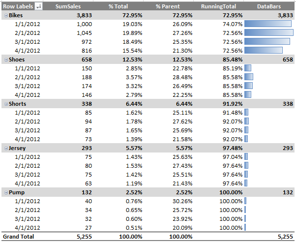
Anyway, here's my simplified use case for this post (sample file here). Let's say I'm a sales analyst for AdventureWorks, and I've got sales data that I want to analyze from several perspectives in one dashboard. I have one calculated measure that I want to slice up by product and date. And then next to that I want to present those same sales values in percentage form. Both percent of Total as well as a percentage of Product. And I also want to display a running total, so I can get a sense of my 80/20. Something like this:
Granted, this viz could be presented with less numbers and more visualizations, but for this exercise, I'm focusing more on the reuse of the measure, and not the viz. I'll focus on the viz side of this in a later post. So work with me here.
For this pivot, all 5 values presented are based on the same measure. Excel makes this type of analysis extremely easy with a native pivot value setting called "Show Values As". If your desired measure is a simple aggregation, you can just drag a base field from the data model (not a calculated measure) and create 5 implicit measures. Then just use the native Excel "Show Value As" feature on each as needed.

The wrinkle in versions prior to 2013 was that Excel wouldn't allow you to use the same calculated measure from a PowerPivot model more than once in the pivot Values area. You could only do this by creating multiple implict measures. And there are definitely scenarios where simple aggregates and implicit measures just won't cut it.
In my example for this post, I needed to multiply units by price at the transaction level to get my sales amount. Can't do that with an implicit measure, because I'm referencing 2 fields. And in my case, lets say my fact table is massive and I can't afford to store units and price plus an additional calculated column for extended amount (I know, simple scenario, but work with me because you will likely run into this for some more complicated calculations). Anyway, in this case and many others, defining calculated measures with some DAX wizardry will be your only hope.

In working through this last year, the only way I could find to get those multiple copies of the calculated measure into the pivot as needed for use with "Show Values As" was to create additional copies of the calculated measure in the model. Or give up and manually build all of the DAX logic into additional measures that Excel's "Show Values As" feature would have given me for free.
Note: that second approach is actually a worthwhile solution when you are delivering these measures through other tools besides Excel that don't have "Show Values As" baked in. But it would also be a lot of work and would add a large number of measures to the model. And for this post, I just want to focus on the Excel - PowerPivot integration perspective.
So, that said, the point of this post is that, when I hit this issue last year, it would have been GLORIOUS to be able to use calculated measures as flexibly as implicit measures with the "Show Values As" feature. And now, in Excel2013, that's exactly what you can do. The product team built that very capability into the new release. And the best part, at least from my limited testing, is that I don't see any implicit measures added to the underlying PowerPivot model. Just apparently a "virtual" copy of the measure for the particular pivot you are referencing it from. Keeps the model nice and tidy. Beautiful stuff. I'm sure there are technical details about the internal implementation that I'm missing here, but for now, I'm coming at this from the user perspective.

So enough description. Here's the actual step-by-step instructions to decompose my example from above. Since I have a very large fact table, to save memory and get better compression, I stored the units and price separately (instead of calculating the extended price as a calculated column on each row). To get the extended Sales amount for my analysis, I created a calculated measure defined as:
SumSales:= SUMX(FactSales, FactSales[Units] * FactSales[Price])
And then, to build the pivot table, I simply drag that measure into the Values area 5 times to create the following:
1. SumSales: Raw measure values
2. % Total: based on measure SumSales
- modify the Custom Name to "% Total"
- modify the field setting for "Show Values As" to "% Grand Total" like below

3. % Parent: based on measure SumSales
- modify the custom name
- set "Show Values As" property to "% Parent Row Total" like below

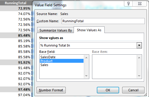
4: RunningTotal: based on measure SumSales
- modify custom name
- set "Show Values As" property to "% Running Total of" Product like below
5. DataBars: based on measure SumSales
- modify custom name
- select a values cell at the product / date level & set conditional formatting for databars
(Home tab -> Conditional Formatting button -> Data Bars)

That last one for Data Bars is particularly useful. Especially since, if you use Data Bars within a cell that has your measure values, the larger numbers will get overlapped by the bar in the cell, making it a bit messy and hard to read. Using 2 copies of the measure instead allows you to use one to display the value and the other to display the bar. Nice and clean.
That's it. Now I've got 5 flavors of my efficient SumSales calculated measure, and have taken advantage of several of Excel's out-of-the-box analysis features. Without having to code all of those measures manually in DAX. If you want to check out my sample workbook, here's a link to it on my SkyDrive.
Let me know if that's helpful.
No comments:
Post a Comment